Transition networks with python

First the imports in ipython notebook:

%pylab inline
import skimage.morphology as morphology
import sklearn.cluster
import graphviz
import os
import PIL
import matplotlib.gridspec as gridspec

Identifying metastable states

Understanding a system’s conformational dynamics can be summed up into two steps:

identifying the long lived, or metastable, states visited by the system
determining the rates of transitioning between these states.

I decided to reproduce in python the results obtained in this publication:

Transition networks for modeling the kinetics of conformational change in macromolecules

by Frank Noé, Stefan Fischer

DOI: 10.1016/j.sbi.2008.01.008

abstract:

The kinetics and thermodynamics of complex transitions in biomolecules can be modeled in terms of a network of transitions between the relevant conformational substates. Such a transition network, which overcomes the fundamental limitations of reaction-coordinate-based methods, can be constructed either based on the features of the energy landscape, or from molecular dynamics simulations. Energy-landscape-based networks are generated with the aid of automated path-optimization methods, and, using graph-theoretical adaptive methods, can now be constructed for large molecules such as proteins. Dynamics- based networks, also called Markov State Models, can be interpreted and adaptively improved using statistical concepts, such as the mean first passage time, reactive flux and sampling error analysis. This makes transition networks powerful tools for understanding large-scale conformational changes.

The 1D energy of the system

x = linspace(0,100,7)
y = [5, 1.5, 4, 1, 2, 1.5,5]

plot(x,y,'o')
z = np.polyfit(x, y, 6)
E = np.poly1d(z)

x_lin = linspace(0, 100, 100)
plot(x_lin,E(x_lin), linewidth=2)
ylabel('Energy ($k_{B}T$)', fontsize=18)
xlabel('discrete coordinates', fontsize=18)
grid()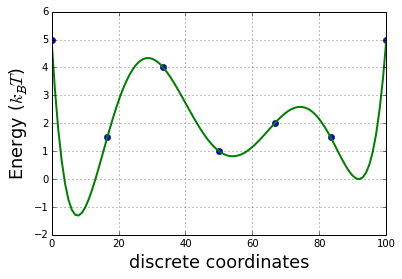

png

This energy plot is sample with a basic Markov Chain Monte Carlo (MCMC)

def montecarlo(potential=E, nstep=1000):
    p = lambda x: exp(-x)
    pos_prev = random.randint(0,100)
    traj = []
    for i in range(nstep):
        pos = pos_prev + randint(0, 2)*2 -1
        while not (0 <= pos < 100):
            pos = pos_prev + randint(0, 2)*2 -1
        delta = potential(pos) - potential(pos_prev)
        if delta > 0:
            #print p(delta)
            if p(delta) < random.uniform():
                pos = pos_prev
            else:
                pos_prev = pos
        else:
            pos_prev = pos
        #print pos, pos_prev, delta, potential(pos), potential(pos_prev)
        traj.append(pos)
    return asarray(traj)

1000000 steps of MCMC and we compute the transition matrix

traj = montecarlo(nstep=1000000)

Here the distribution obtained with th MCMC which fit quite well the energy plot

tmp = hist(traj, 100, normed=True)
ylabel('$\pi$', fontsize=18)
xlabel('discrete coordinates', fontsize=18)
grid()

def get_transition_matrix(traj, lag=1):
    T = zeros((100, 100))
    density = zeros(100, dtype=int)
    for e in zip(traj, traj[lag:]):
        i,j = e
        T[i,j] += 1
        density[i] += 1
    T /= density
    return nan_to_num(T)
T = get_transition_matrix(traj, lag=200)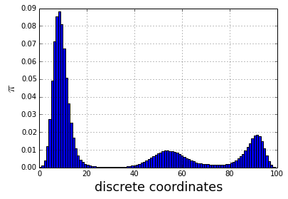

png

The plot of the transition matrix

imshow(T, interpolation='nearest', cmap=cm.coolwarm, norm=matplotlib.colors.LogNorm())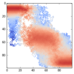

png

The transition matrix is then diagonalized

w,v = linalg.eig(T)
w = real(w)
v = real(v)
v = v[:,w.argsort()[::-1]]
w = w[w.argsort()[::-1]]

Just a simple watershed on the energy to identify energy basins based on the energy plot

structelem = numpy.ones((3), dtype='bool')
labels = zeros(100)
for i,e in enumerate(x[1:6:2]):
    labels[int(e)] = i+1
x_lin = linspace(0, 100, 100)
labels_full = morphology.watershed(E(x_lin), labels, connectivity=structelem)

A function to substitute values in an array

def substitute(d, arr):
    """
    d: {0: 3, 1: 1, 2: 2} for example: values to substitute
    """
    new_arr = copy.deepcopy(arr)
    for i, j in d.iteritems(): 
        new_arr[arr==i] = j
    return new_arr

The projection of the transition matrix onto the second and third eigen vector

proj = dot(transpose(T),v[:,1:3])
# create k-meansclustering estimators
kmeans = sklearn.cluster.KMeans(n_clusters=3)
kmeans.fit(proj)
mgrid = asarray(meshgrid(linspace(min(proj[:,0]),max(proj[:,0]),100),linspace(min(proj[:,1]),max(proj[:,1]),100))).T
kmeans_partition = kmeans.predict(mgrid.reshape(100*100,2)).reshape(100,100)
d = {}
for i in unique(kmeans.labels_):
    c,b = histogram(labels_full[kmeans.labels_==i])
    d[i] = int(b[argmax(c)])
print d
imshow(kmeans_partition[:,::-1].T, interpolation='none', extent=[min(proj[:,0]),max(proj[:,0]),min(proj[:,1]),max(proj[:,1])])
colorbar()
scatter(proj[:,0], proj[:,1],c=labels_full, s=64)
xlabel('second eigenvector')
ylabel('third eigenvector')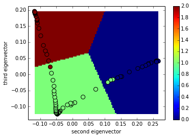

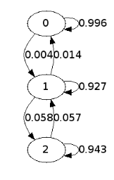
png

The code below identifies the three metastable states and compute the Markov chain model

pi, bins = histogram(traj, normed=True, bins=100)
plot(pi)
xlabel('discrete coordinates', fontsize = 18)
ylabel('$\pi$', fontsize=18)
def meta_transition(c1,c2):
    sel1 = kmeans.labels_ == c1
    sel2 = kmeans.labels_ == c2
    ind1 = where(sel1)[0]
    ind2 = where(sel2)[0]
    num = 0
    for i in ind1:
        for j in ind2:
            num+=pi[i] * T[j,i]
    trans = num/pi[sel1].sum()
    return trans

gdot = graphviz.Digraph()
for i in unique(kmeans.labels_):
    gdot.node('%d'%i)
for i in unique(kmeans.labels_):
    for j in unique(kmeans.labels_):
        weight = meta_transition(i,j)
        if weight > 0:
            gdot.edge('%d'%i, '%d'%j, label='%.3f'%weight)
            
dotfn = 'graph.dot'    
gdot.render(filename=dotfn)

def plotdotgraph(dotfn):
    os.system('dot -T png -o %s.png %s'%(dotfn,dotfn))
    img = PIL.Image.open('%s.png'%dotfn)
    imshow(img)
    axis('off')

figure()
tmp = plotdotgraph(dotfn)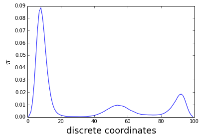

png

And here the full story in one plot:

rcParams['figure.figsize'] = 18,10

gs = gridspec.GridSpec(4,3, height_ratios=(1,1,1,3))
gs.update(hspace=.5)

subplot(gs[:3,0])
x_lin = linspace(0, 100, 100)
for i in range(3):
    plot(x_lin[labels_full==i+1],E(x_lin)[labels_full==i+1], linewidth=2)
ylabel('Energy ($k_{B}T$)', fontsize=18)
xlabel('discrete coordinates', fontsize=18)
grid()

subplot(gs[:3,1])
imshow(T, interpolation='nearest', cmap=cm.coolwarm, norm=matplotlib.colors.LogNorm())

for i in range(3):
    subplot(gs[i,2])
    for j in range(3):
        plot(x_lin[labels_full==j+1],-v[:,i][labels_full==j+1], linewidth=2)
    grid()
xlabel('discrete coordinates', fontsize=18)

subplot(gs[3,0])
plot(w[:10], 'o--')
xlabel('eigenvalue index', fontsize=18)
ylabel('eigenvalue', fontsize=18)
grid()

subplot(gs[3,1])
imshow(kmeans_partition[:,::-1].T, interpolation='none', extent=[min(proj[:,0]),max(proj[:,0]),min(proj[:,1]),max(proj[:,1])],
       alpha=.5)
scatter(proj[:,0], proj[:,1],c=labels_full, s=64)
xlabel('second eigenvector', fontsize=18)
ylabel('third eigenvector', fontsize=18)
grid()

subplot(gs[3,2])
plotdotgraph(dotfn)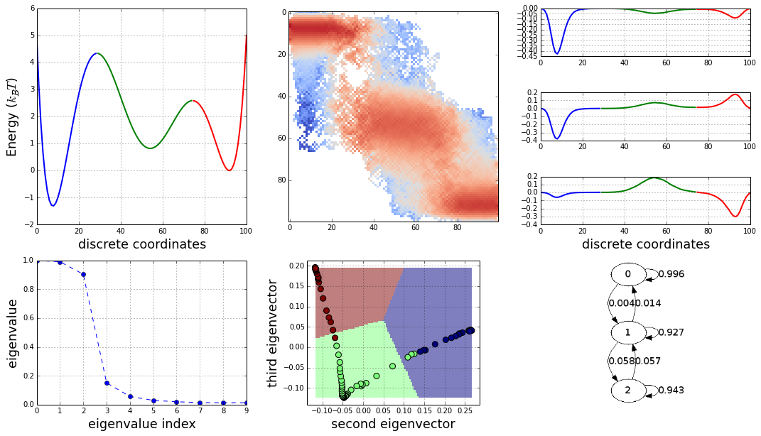

png

The construction of a transition network. (a) Sample potential, defined over a one-dimensional coordinate that is discretized into 100 microstates. It has three metastable basins (0 (blue), 1 (green), and 2 (red)). (b) Transition matrix T for a Markov lagtime of 200 steps. The transition probability was obtained from a Metropolis Monte Carlo, jumping each step only to the current or adjacent microstates. T exhibits three clusters corresponding to the metastable states. (c) Left eigenvectors of T indicating the transition modes among microstates. The first eigenvector gives the stationary distribution. The sign structure of the second eigenvector partitions the state space into two metastable states, blue and red. The sign structure of the third eigenvector further splits green and red, obtaining three metastable states. (d) The eigenvalue spectrum of T. The clear gaps after 2 and 3 eigenvalues indicate how many states are metastable. (e) Coordinates of the 100 microstates projected onto the second and third right eigenvectors of T. Metastable states are identified by clustering the microstates in this eigenspace. (f) Transition network between the 3 metastable states A, B and C

The caption is adapted from: Transition networks for modeling the kinetics of conformational change in macromolecules

If you want to ask me a question or leave me a message add @bougui505 in your comment.