Simple Markov chain Monte Carlo (MCMC) algorithm in python
I present here a simple Markov chain Monte Carlo python implementation to sample a 2D surface of potential.
%pylab inlineFirst I define a Müller potential from a piece of code I found on gist.
def muller_potential(x, y, use_numpy=False):
    """Muller potential
    Parameters
    ----------
    x : {float, np.ndarray, or theano symbolic variable}
    X coordinate. If you supply an array, x and y need to be the same shape,
    and the potential will be calculated at each (x,y pair)
    y : {float, np.ndarray, or theano symbolic variable}
    Y coordinate. If you supply an array, x and y need to be the same shape,
    and the potential will be calculated at each (x,y pair)

    Returns
    -------
    potential : {float, np.ndarray, or theano symbolic variable}
    Potential energy. Will be the same shape as the inputs, x and y.
    Reference
    ---------
    Code adapted from https://cims.nyu.edu/~eve2/ztsMueller.m
    """
    aa = [-1, -1, -6.5, 0.7]
    bb = [0, 0, 11, 0.6]
    cc = [-10, -10, -6.5, 0.7]
    AA = [-200, -100, -170, 15]
    XX = [1, 0, -0.5, -1]
    YY = [0, 0.5, 1.5, 1]
    # use symbolic algebra if you supply symbolic quantities
    exp = np.exp
    value = 0
    for j in range(0, 4):
        if use_numpy:
            value += AA[j] * numpy.exp(aa[j] * (x - XX[j])**2 + bb[j] * (x - XX[j]) * (y - YY[j]) + cc[j] * (y - YY[j])**2)
        else: # use sympy
            value += AA[j] * sympy.exp(aa[j] * (x - XX[j])**2 + bb[j] * (x - XX[j]) * (y - YY[j]) + cc[j] * (y - YY[j])**2)
    return value
Which looks like:
minx=-1.5
maxx=1.2
miny=-0.2
maxy=2
ax=None
grid_width = max(maxx-minx, maxy-miny) / 200.0
xx, yy = np.mgrid[minx : maxx : grid_width, miny : maxy : grid_width]
V = muller_potential(xx, yy, use_numpy=True)
contourf(xx, yy, ma.masked_array(V.clip(max=200), V>inf), 40)
tmp = colorbar()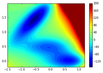
The code for MCMC sampling is quite short:
def montecarlo(potential=V, nstep=1000, beta=1, markov=True):
    p = lambda x: exp(-beta*x)
    nx,ny = potential.shape
    pos_prev = (np.random.randint(0,nx), np.random.randint(0,ny))
    traj = []
    for i in range(nstep):
        if markov:
            pos = (pos_prev + asarray([random.choice([-1,0,1]), random.choice([-1,0,1])]))%(nx,ny)
        else:
            pos = (np.random.randint(0,nx), np.random.randint(0,ny))
        pos = tuple(pos)
        pos_prev = tuple(pos_prev)
        delta = potential[pos] - potential[pos_prev]
        if delta > 0:
            #print p(delta)
            if p(delta) < np.random.uniform():
                pos = pos_prev
            else:
                pos_prev = pos
        else:
            pos_prev = pos
        traj.append(pos)
    return asarray(traj)
And takes less than 1 minute for 1 000 000 steps of monte carlo:
nstep=1000000
traj = montecarlo(nstep=nstep, beta=0.125, markov=False)

density = zeros_like(V)
for pos in traj:
    pos = tuple(pos)
    density[pos] += 1
Now we can plot the distribution obtained onto the surface of the potential sampled:
contour(V.clip(max=200), 15)
imshow(density / nstep, cmap=cm.coolwarm, norm=matplotlib.colors.LogNorm())
tmp = colorbar()
And if you increase :
nstep=1000000
traj = montecarlo(nstep=nstep, beta=0.025, markov=False)

density = zeros_like(V)
for pos in traj:
    pos = tuple(pos)
    density[pos] += 1
You sample more:
contour(V.clip(max=200), 15)
imshow(density / nstep, cmap=cm.coolwarm, norm=matplotlib.colors.LogNorm())
tmp = colorbar()