Metadynamics on a 2D surface potential with python

First, the python import in the ipython notebook:

%pylab inline
import matplotlib.gridspec as gridspec
import scipy.spatial.distance
from skimage.feature import peak_local_max
import scipy.ndimage.filters
import copy
from matplotlib import animation
from JSAnimation import IPython_display
from JSAnimation.IPython_display import display_animation

Populating the interactive namespace from numpy and matplotlib

As usual, we define the Müller potential as the sampled potential:

def muller_potential(x, y):
    """Muller potential
    Parameters
    ----------
    x : {float, np.ndarray, or theano symbolic variable}
    X coordinate. If you supply an array, x and y need to be the same shape,
    and the potential will be calculated at each (x,y pair)
    y : {float, np.ndarray, or theano symbolic variable}
    Y coordinate. If you supply an array, x and y need to be the same shape,
    and the potential will be calculated at each (x,y pair)
    Returns
    -------
    potential : {float, np.ndarray, or theano symbolic variable}
    Potential energy. Will be the same shape as the inputs, x and y.
    Reference
    ---------
    Code adapted from https://cims.nyu.edu/~eve2/ztsMueller.m
    """
    aa = [-1, -1, -6.5, 0.7]
    bb = [0, 0, 11, 0.6]
    cc = [-10, -10, -6.5, 0.7]
    AA = [-200, -100, -170, 15]
    XX = [1, 0, -0.5, -1]
    YY = [0, 0.5, 1.5, 1]
    # use symbolic algebra if you supply symbolic quantities
    exp = np.exp
    value = 0
    for j in range(0, 4):
        value += AA[j] * numpy.exp(aa[j] * (x - XX[j])**2 + bb[j] * (x - XX[j]) * (y - YY[j]) + cc[j] * (y - YY[j])**2)
    return value

2D plot of the sampled potential:

minx=-1.5
maxx=1.2
miny=-0.2
maxy=2
ax=None
grid_width = max(maxx-minx, maxy-miny) / 200.0
xx, yy = np.mgrid[minx : maxx : grid_width, miny : maxy : grid_width]
V = muller_potential(xx, yy)
contourf(xx, yy, V.clip(max=200), 40)
colorbar()

<matplotlib.colorbar.Colorbar instance at 0xd54d3f8>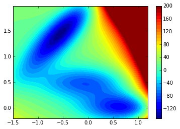

png

Now, we search for the 3 local minima of the potential defined:

print xx.shape
local_minima_grid = peak_local_max(-V)
local_minima = []
for e in local_minima_grid:
    local_minima.append([xx[tuple(e)], yy[tuple(e)]])
local_minima = asarray(local_minima)

(200, 163)

contourf(xx, yy, V.clip(max=200), 40)
colorbar()
scatter(local_minima[:,0], local_minima[:,1], c='r')

<matplotlib.collections.PathCollection at 0xd96d910>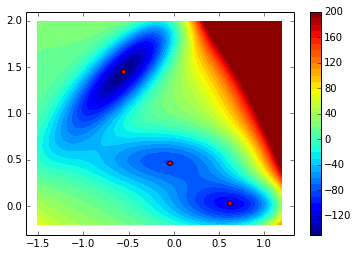

png

And now the standard MCMC sampler:

def montecarlo(start=None,potential=V, nstep=1000, beta=1, markov=True):
    p = lambda x: exp(-beta*x)
    nx,ny = potential.shape
    if start == None:
        pos_prev = (np.random.randint(0,nx), np.random.randint(0,ny))
    else:
        pos_prev = start
    traj = []
    for i in range(nstep):
        if markov:
            pos = (pos_prev + asarray([random.choice([-1,0,1]), random.choice([-1,0,1])]))%(nx,ny)
        else:
            pos = (np.random.randint(0,nx), np.random.randint(0,ny))
        pos = tuple(pos)
        pos_prev = tuple(pos_prev)
        delta = potential[pos] - potential[pos_prev]
        if delta > 0:
            #print p(delta)
            if p(delta) < np.random.uniform():
                pos = pos_prev
            else:
                pos_prev = pos
        else:
            pos_prev = pos
        traj.append(pos)
    return asarray(traj)

The sampling:

nstep=100000
traj = montecarlo(start = local_minima_grid[2], nstep=nstep, beta=1, markov=True)

And the distribution obtained:

def get_density(traj):
    density = zeros_like(V)
    for pos in traj:
        pos = tuple(pos)
        density[pos] += 1
    return density
density = get_density(traj)

contour(V.clip(max=200), 15)
imshow(density / nstep, cmap=cm.coolwarm, norm=matplotlib.colors.LogNorm())
tmp = colorbar()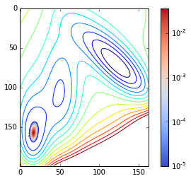

png

Now, we define a Gaussian for the sampling by metadynamics:

def Gaussian(x,y,x0,y0,w=1,sigma=1):
    Z = w*numpy.exp(- ((x-x0)**2 + (y-y0)**2) / (2*sigma**2))
    return Z

And the MCMC sampler is modified to add a Gaussian at each point visited during the sampling:

def metamontecarlo(start = None, potential=V, nstep=1000, beta=1, markov=True):
    potential_flooding = []
    p = lambda x: exp(-beta*x)
    nx,ny = potential.shape
    if start == None:
        pos_prev = (np.random.randint(0,nx), np.random.randint(0,ny))
    else:
        pos_prev = start
    traj = []
    for i in range(nstep):
        if markov:
            pos = (pos_prev + asarray([random.choice([-1,0,1]), random.choice([-1,0,1])]))%(nx,ny)
        else:
            pos = (np.random.randint(0,nx), np.random.randint(0,ny))
        pos = tuple(pos)
        pos_prev = tuple(pos_prev)
        delta = potential[pos] - potential[pos_prev]
        if delta > 0:
            #print p(delta)
            if p(delta) < np.random.uniform():
                pos = pos_prev
            else:
                pos_prev = pos
        else:
            pos_prev = pos
        potential += Gaussian(xx,yy, xx[pos],yy[pos], w=0.01, sigma=10*grid_width)
        #potential_k = copy.deepcopy(potential)
        #potential_flooding.append(potential_k)
        traj.append(pos)
    return asarray(traj)#, asarray(potential_flooding)

Now we sample with the same parameters beta and nstep but with the ‘Gaussian flooding’

nstep=100000
potential = copy.deepcopy(V)
traj = metamontecarlo(start = local_minima_grid[2], potential=potential, nstep=nstep, beta=1, markov=True)
density = zeros_like(V)
for pos in traj:
    pos = tuple(pos)
    density[pos] += 1

save('traj_meta', traj)

traj_meta = load('traj_meta.npy')

Now we’ll use the JSAnimation module to generate an animation of the sampling:

fig = plt.figure()
axis('off')
potential_flood = copy.deepcopy(V)
nx,ny = potential.shape
ims = []
for k in range(nstep):
    pos = tuple(traj_meta[k])
    potential_flood += Gaussian(xx,yy, xx[pos],yy[pos], w=0.01, sigma=10*grid_width)
    if k%100 == 0:
        potential_k = copy.deepcopy(potential_flood)
        for i in range(3):
            for j in range(3):
                u, v = pos[0]+i, pos[1]+j
                if u < nx and v < ny:
                    potential_k[u,v] = 200
        im = plt.imshow(potential_k, interpolation='nearest', vmin = V.min(), vmax=200)
        ims.append([im])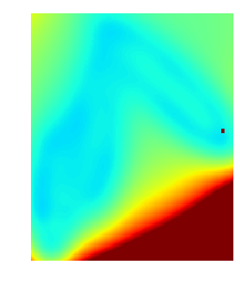

png

animation.ArtistAnimation(fig, ims, interval=50, blit=True,
    repeat_delay=1000)

Below, just some snapshots of the metadynamics and standard sampling for comparison:

max_density_meta = get_density(traj_meta).max()
max_density = get_density(traj).max()

potential_flood = copy.deepcopy(V)
nx,ny = potential.shape
potential_flooding = []
for k in range(nstep):
    pos = tuple(traj_meta[k])
    potential_flood += Gaussian(xx,yy, xx[pos],yy[pos], w=0.01, sigma=10*grid_width)
    if k%10000 == 0:
        potential_k = copy.deepcopy(potential_flood)
        potential_flooding.append(potential_k)

print len(potential_flooding)

rcParams['figure.figsize'] = 16,12
gs=gridspec.GridSpec(4,6)
bg1 = zeros((nx,ny,3))
bg1[:,:,0] = 1
bg2 = zeros((nx,ny,3))
bg2[:,:,1] = 1
u=0
v=0
trajs = []
trajs_meta= []
delta = 10000
for i,c in enumerate(range(0,nstep,delta)):
    trajs.append(traj[i*delta:(i+1)*delta])
    subtraj = asarray(trajs).reshape((i+1)*delta,2)
    sub_density = get_density(subtraj)
    subplot(gs[u+1,v])
    imshow(bg2, alpha=.25)
    contour(V.clip(max=200), 15, vmin=V.min(), vmax=200)
    imshow(sub_density/max_density, cmap=cm.coolwarm, norm=matplotlib.colors.LogNorm(), interpolation='nearest', vmax=1)
    axis('off')
    #starts = starts_list[i]
    
    subplot(gs[u,v])
    imshow(bg1, alpha=.25)
    contour(potential_flooding[i].clip(max=200), 15, vmax=200)
    trajs_meta.append(traj_meta[i*delta:(i+1)*delta])
    subtraj_meta = asarray(trajs_meta).reshape((i+1)*delta,2)
    sub_density_meta = get_density(subtraj_meta)
    imshow(sub_density_meta/max_density_meta, cmap=cm.coolwarm, norm=matplotlib.colors.LogNorm(), interpolation='nearest', vmax=1)
    title('%d steps'%((i+1)*delta))
    axis('off')
    v+=1
    if v == 5:
        subplot(gs[u,v])
        text(0,0.5,'Metadynamics', fontsize=14)
        axis('off')
        subplot(gs[u+1,v])
        text(0,0.5,'Standard sampling', fontsize=14)
        axis('off')
        v = 0
        u += 2
savefig('metadynamics.png', dpi=300, bbox_inches='tight' )

png

If you want to ask me a question or leave me a message add @bougui505 in your comment.