Smoothed data histogram with SOM
I played a lot with Self-Organizing Map (SOM). The 2D SOM distributes the input vectors onto a 2D plane. Mathematically the SOM is a 3D matrix and the length of the third dimension is given by the length of your input data. To visualize the SOM it’s usual to compute the Unified distance matrix (U-matrix). The U-matrix gives for each neuron of the SOM the mean Euclidean distance between the considered neuron and its neighbors.
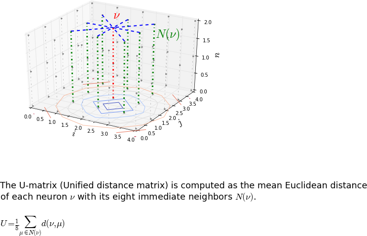
Another way to visualize the SOM is to count the number of input data in each bin of the SOM. However the SOM algorithm try to sparse data homogeneously within the map. The basic idea here is to smooth the histogram of the SOM. To do this each input data is not attributed to a unique cell but to an ensemble of cells. The number of cells in the ensemble is determined by the smoothing parameter . This idea come from this document: Using Smoothed Data Histograms for Cluster Visualization in Self-Organizing Maps.
The ipython notebook import:
%pylab inline
import scipy.ndimage
import random
import sys
sys.path.append('/Bis/home/bougui/bin/SOM')
import SOM2
import SOMclust
import scipy.spatial.distance
from mpl_toolkits.mplot3d import Axes3D
rcParams['figure.figsize'] = 10,6
A 2D potential constructed from 4 randomly chosen points.
E = ones((50,50))
pos = [(10,10),(30,40),(40,10),(10,40)]
for c in pos:
    E[c] = 0
E = scipy.ndimage.morphology.distance_transform_edt(E)
matshow(E, cmap=cm.coolwarm)
tmp = colorbar()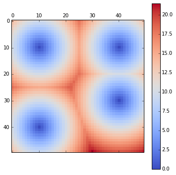
This potential is then sampled using a Monte-Carlo
def montecarlo(potential=E, nstep=1000, beta=1, markov=True):
    p = lambda x: exp(-beta*x)
    nx,ny = potential.shape
    pos_prev = (np.random.randint(0,nx), np.random.randint(0,ny))
    traj = []
    for i in range(nstep):
        if markov:
            pos = (pos_prev + asarray([random.choice([-1,0,1]), random.choice([-1,0,1])]))%(nx,ny)
        else:
            pos = (np.random.randint(0,nx), np.random.randint(0,ny))
        pos = tuple(pos)
        pos_prev = tuple(pos_prev)
        delta = potential[pos] - potential[pos_prev]
        if delta > 0:
            #print p(delta)
            if p(delta) < np.random.uniform():
                pos = pos_prev
            else:
                pos_prev = pos
        else:
            pos_prev = pos
        traj.append(pos)
    return asarray(traj)

nstep=50000
traj = montecarlo(nstep=nstep, beta=0.25, markov=False)

density = zeros_like(E)
for pos in traj:
    pos = tuple(pos)
    density[pos] += 1
And then we plot the distributions obtained from the MCMC:
matshow(density / nstep, cmap=cm.coolwarm, norm=matplotlib.colors.LogNorm())
tmp = colorbar()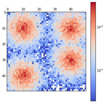
A Self-organizing map is trained with the MCMC sampling:
som = SOM2.SOM(traj)
tmp = som.learn()
The resulting U-matrix.
(Here I used a algorithm to unwrap the U-matrix as the SOM is chosen with periodic boundaries. The visualization is simpler with this representation.)
The gray scale dots are the original density of the data in the SOM space.
umat = som.umatrix()

som_density = zeros_like(som.smap[:,:,0])
bmus = som.get_allbmus()
for e in bmus:
    som_density[tuple(e)]+=1

clust = SOMclust.clusters(umat, bmus, som.smap)

contour(ma.masked_array(clust.umat_cont, clust.mask), 20, interpolation='nearest')
tmp = axis('off')
density_cont = clust.flood(som_density)[0]
imshow(ma.masked_array(density_cont, clust.mask), interpolation='nearest', cmap=cm.gray_r)
tmp = axis('off')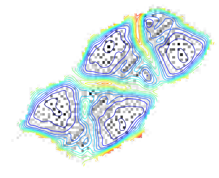
And the U-matrix in the input space in comparison with the 2D histogram of the input data:
subplot(120)
c = umat.flatten()
scatter(som.smap[:,:,1].flatten()[c.argsort()[::-1]], som.smap[:,:,0].flatten()[c.argsort()[::-1]],
        c=c[c.argsort()[::-1]], linewidths=0, cmap=cm.coolwarm, marker='s')
subplot(121)
input_dist = asarray(meshgrid(range(50), range(50))).T.reshape(2500,2)
scatter(input_dist[:,1], input_dist[:,0], c=density, linewidths=0, cmap=cm.gray_r, marker='s')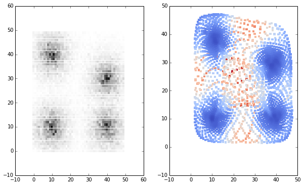
Now we compute the smooth data histogram (SDH). The membership degree is to the closest bin, to the second, to the third and so forth. The membership to all but the closest bins is 0. is defined as:
def sdh(smap, inputmat, s=8):
    """
    return the smooth data histogram of the SOM density
    """
    x,y,n = smap.shape
    sdhmat = zeros(x*y)
    dmat = scipy.spatial.distance.cdist(inputmat, smap.reshape(x*y,n))
    #hmat = dmat.argsort(axis=1)[:,:s] # hit matrix
    c = float(arange(1,s+1).sum())
    for ds in dmat:
        l = argsort(ds)[:s]
        for i,ind in enumerate(l):
            sdhmat[ind] += (s-i)/c
    sdhmat = sdhmat.reshape((x,y))
    return sdhmat
For large dataset you can run out of memory when you compute the full distance matrix dmat with scipy.spatial.distance.cdist(inputmat, smap.reshape(x*y,n)).
Instead of computing dmat you can use KDTree or cKDTree.
This class provides an index into a set of k-dimensional points which can be used to rapidly look up the nearest neighbors of any point.
In the function below I’ve also added the data parameter to project a weighted sum of the data with the rule exposed before.
def sdh(smap, inputmat, s=8, data=None):
    """
    Return the smooth data histogram of the SOM density.
    If data is not None return the smoothed projection of the data onto the map
    """
    x,y,n = smap.shape
    sdhmat = zeros(x*y)
    kdtree = scipy.spatial.cKDTree(smap.reshape(x*y,n))
    c = float(arange(1,s+1).sum())
    ds,ls = kdtree.query(inputmat,k=s)
    for i,d in enumerate(ds):
        l = ls[i]
        for j,ind in enumerate(l):
            if data == None:
                sdhmat[ind] += (s-j)/c
            else:
                sdhmat[ind] += (s-j)*data[i]/c
    sdhmat = sdhmat.reshape((x,y))
    return sdhmat
I’ve slightly changed the function to apply a distance cutoff
distances_threshold instead of a cutoff on the number of bins ():
def sdh(smap, inputmat, s=8, distances_threshold=None, data=None):
    """
    Return the smooth data histogram of the SOM density.
    If data is not None return the smoothed projection of the data onto the map
    If distances_threshold is not none apply a distance cutoff instead of a fix number of cells
    """
    x,y,n = smap.shape
    sdhmat = zeros(x*y)
    kdtree = scipy.spatial.cKDTree(smap.reshape(x*y,n))
    c = float(arange(1,s+1).sum())
    if distances_threshold == None:
        ds,ls = kdtree.query(inputmat,k=s)
        for i,d in enumerate(ds):
            l = ls[i]
            for j,ind in enumerate(l):
                if data == None:
                    sdhmat[ind] += (s-j)/c
                else:
                    sdhmat[ind] += (s-j)*data[i]/c
    else:
        for v in inputmat:
            l = kdtree.query_ball_point(v, distances_threshold)
            s = len(l)
            c = float(arange(1,s+1).sum())
            for j, ind in enumerate(l):
                if data == None:
                    sdhmat[ind] += (s-j)/c
                else:
                    sdhmat[ind] += (s-j)*data[i]/c
    sdhmat = sdhmat.reshape((x,y))
    return sdhmat
And we choose a smoothing parameter s of 16
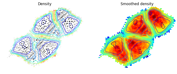
sdhmat = sdh(som.smap,traj, s=16)We compare below the original density and the smoothed density:
subplot(121)
imshow(ma.masked_array(density_cont, clust.mask), interpolation='nearest', cmap=cm.gray_r)
contour(ma.masked_array(clust.umat_cont, clust.mask), 10, interpolation='nearest')
title('Density')
tmp = axis('off')
subplot(122)
sdhmat_cont = clust.flood(sdhmat)[0]
imshow(ma.masked_array(sdhmat_cont, clust.mask), interpolation='nearest', norm=matplotlib.colors.LogNorm(), cmap=cm.jet)
contour(ma.masked_array(clust.umat_cont, clust.mask), 10, interpolation='nearest')
title('Smoothed density')
tmp = axis('off')