Elastic network model of proteins with python

I used this two documents to write this post:

Low-frequency normal modes of proteins. Yves-Henri Sanejouand. Biological Physics. Université Claude Bernard - Lyon I, 2007. In french.
Normal mode theory and harmonic potential approximations. Konrad Hinsen

Other documents of interest:

A harmonic potential well has the form:

$U(r) = \frac{1}{2}(r-R) \cdot K(r) \cdot (r-R)$

with $R$ a $3N$ dimensional vector ( $N$ is the number of atoms) of the stable conformation and $r$ the same object of the current conformation.

$K$ is the Hessian matrix of $U$ :

$K_{ij} = \frac{\partial^2 U}{\partial r_{i} \partial r_{j}}$

and:

$U = \frac{1}{2} k(\|r_i - r_j\|-\|R_i-R_j\|)^2$

We denote:

$s_{ij} = \|r_i-r_j\|$

and

$s_{ij}^o = \|R_i-R_j\|$

Now we can define the second derivative of $V$ :

${\partial^2 V_{ij}\over\partial{x_i}^2} = {k\over {s_{ij}}^2} {(x_j - x_i)}^2$

and

${\partial^2 V_{ij}\over\partial x_i\partial y_j} = {-k\over {s_{ij}}^2} {(x_j - x_i)}{(y_j-y_i)}$

which allows us to define the Hessian matrix $K$ :

$K_{ij} = \begin{bmatrix} {\partial^2 V_{ij}\over\partial x_i\partial x_j} & {\partial^2 V_{ij}\over\partial x_i\partial y_j} & {\partial^2 V_{ij}\over\partial x_i\partial z_j} \\ {\partial^2 V_{ij}\over\partial y_i\partial x_j} & {\partial^2 V_{ij}\over\partial y_i\partial y_j} & {\partial^2 V_{ij}\over\partial y_i\partial z_j} \\ {\partial^2 V_{ij}\over\partial z_i\partial x_j} & {\partial^2 V_{ij}\over\partial z_i\partial y_j} & {\partial^2 V_{ij}\over\partial z_i\partial z_j}\end{bmatrix}$

as:

$K_{ij} = {-k\over {s_{ij}}^2} \begin{bmatrix} {(x_j - x_i)(x_j - x_i)} & {(x_j - x_i)(y_j - y_i)} & {(x_j - x_i)(z_j - z_i)} \\ {(y_j - y_i)(x_j - x_i)} & {(y_j - y_i)(y_j - y_i)} & {(y_j - y_i)(z_j - z_i)} \\{(z_j - z_i)(x_j - x_i)} & {(z_j - z_i)(y_j - y_i)} & {(z_j - z_i)(z_j - z_i)} \end{bmatrix}$

Which can then be written as,

$K_{ij} = {-k\over {s_{ij}}^2} \begin{bmatrix} x_j - x_i\\y_j - y_i\\z_j-z_i \end{bmatrix} \begin{bmatrix} x_j - x_i & y_j - y_i & z_j-z_i \end{bmatrix}$

The diagonal of $K$ is defined with:

$a_{ii} = -\sum_{j \neq i} a_{ij}$

Now we can play with python, a protein, and normal modes. First the import:

import sys
sys.path.append('/home/bougui/SOM')
import IO
import scipy.spatial
from mpl_toolkits.mplot3d import Axes3D
%pylab inline

And we load the pdb structure with only $C_\alpha$ atoms.

struct = IO.Structure('data/1E4E-prot-CA.pdb')

Now we extract the coordinates of the $C_\alpha$ atoms ( $R$ ):

R = struct.atoms['coord']

Then $s_{ij}^2$ is computed with scipy.spatial and we define a function to compute the Hessian matrix as defined below. We put a distance cutoff of 15 Angstrom.

def supersum(K,i):
    a = zeros((3,3))
    N = K.shape[0]/3
    for j in range(N):
        a+=K[i*3:i*3+3,j*3:j*3+3]
    return a

def supertrace(K,i,j):
    return trace(K[i*3:i*3+3,j*3:j*3+3])

def hessian(R):
    s_squared = scipy.spatial.distance.squareform(scipy.spatial.distance.pdist(R, metric='sqeuclidean'))
    nr,nc = s_squared.shape
    N = nr # number of atom: nr = nc
    K = zeros((N*3,N*3))
    for i in range(N):
        for j in range(i+1,N):
            xyz_i, xyz_j = R[i], R[j]
            d_xyz = xyz_j - xyz_i
            if s_squared[i,j] < 15**2:
                K[i*3:i*3+3,j*3:j*3+3] = -dot(d_xyz[:,None],d_xyz[:,None].T) / s_squared[i,j]
    K += K.T
    for i in range(N):
        a = supersum(K,i)
        K[i*3:i*3+3,i*3:i*3+3] = -a
    return K


rcParams['figure.figsize'] = 8,8
K = hessian(R)
imshow(K, cmap=cm.PRGn, interpolation='nearest', vmin=-1, vmax=1)
tmp = colorbar()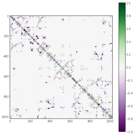

png

And then we diagonalize the Hessian matrix $K$ above:

w,v = eig(K)
v = v[:,w.argsort()]
w = w[w.argsort()]

The sorted eigenvalues $\lambda$ are plotted:

rcParams['figure.figsize'] = 8,4
plot(w, linewidth=2)
xlabel('eigenvalue index', fontsize=14)
ylabel('$\lambda$', fontsize=18)
grid()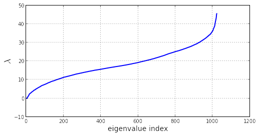

png

The first 6 eigenvalues are null (the 6 degrees of freedom of a rigid body in a 3D space):

plot(w[:20], linewidth=2)
xlabel('eigenvalue index', fontsize=14)
ylabel('$\lambda$', fontsize=18)
grid()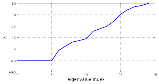

png

Then, we can compute the covariance and correlation matrix from the inverse of the Hessian matrix $K$ :

$K^{-1} = \sum_{i=7}^{3N} \frac{v_{i} \cdot v_{i}^{T}}{\lambda_{i}}$

with $N$ the number of considered atoms.

N = K.shape[0]/3
hessian_inv = zeros((3*N,3*N))
for i in range(6,3*N):
    hessian_inv += (dot(v[:,i][:,None],v[:,i][:,None].T)/w[i])

The element of the covariance matrix is given by the trace of each $3 \times 3$ super element of $K$ . The diagonal of the covariance matrix give the amplitude of the fluctuation for each considered atom of the system.

rcParams['figure.figsize'] = 5,10
cov = zeros((N,N))
for i in range(N):
    for j in range(N):
        cov[i,j] = supertrace(hessian_inv,i,j)
d = cov.diagonal()
subplot(211)
plot(d)
xlabel('sequence of considered atoms', fontsize=14)
ylabel('Amplitude of the fluctuation', fontsize=14)
grid()
corr = cov / sqrt(dot(d[None,:].T,d[None,:]))
subplot(212)
imshow(corr, vmax=0.2)
title('Correlation matrix', fontsize=14)
tmp = colorbar()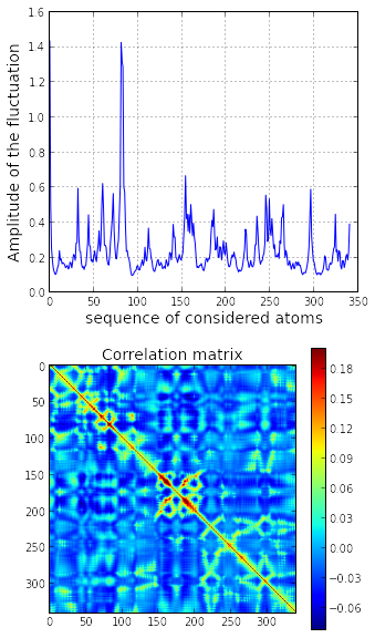

png

Now we can plot the first and the second mode on the structure. First I align the protein on the three axes of inertia:

R-=R.mean(axis=0)
c,a = linalg.eig(dot(R.T,R))
R = dot(R,a)

And, here the plot for the first and second normal mode:

def plot_mode(w, v, mode, cte = 50,doplot=False):
    samples = R
    samples -= samples.mean(axis=0)
    N,dim = samples.shape
    if doplot:
        fig = plt.figure(figsize=(10,10))
        ax = fig.add_subplot(111, projection='3d')
        ax.plot(samples[:,0], samples[:,1], samples[:,2], '-', markersize=10, color='green', lw=1)
        ax.scatter(samples[:,0], samples[:,1], samples[:,2], c=range(samples.shape[0]), marker='o', s=64)
    pc = v[:,mode].reshape(N,3)
    w = sqrt(w[mode])
    nstep=100
    ts = linspace(-w*cte, w*cte, nstep)
    interpolation=zeros((nstep,N*3))
    for j,t in enumerate(ts):
        interpolation[j] = samples.flatten() + t*pc.flatten()
    interpolation = interpolation.reshape(nstep,N,3)
    save('interpolation', interpolation)
    for j,v in enumerate(pc):
        x1,y1,z1 = samples[j]
        x2,y2,z2 = x1+cte*w*v[0], y1+cte*w*v[1], z1+cte*w*v[2]
        if doplot:
            ax.plot([x1,x2], [y1,y2], [z1,z2], color='red', alpha=0.8, lw=2)
    return pc


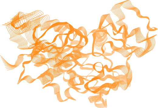
tmp = plot_mode(w, v, 6, doplot=True)
title('Normal mode #1')
tmp = plot_mode(w, v, 7, doplot=True)
title('Normal mode #2')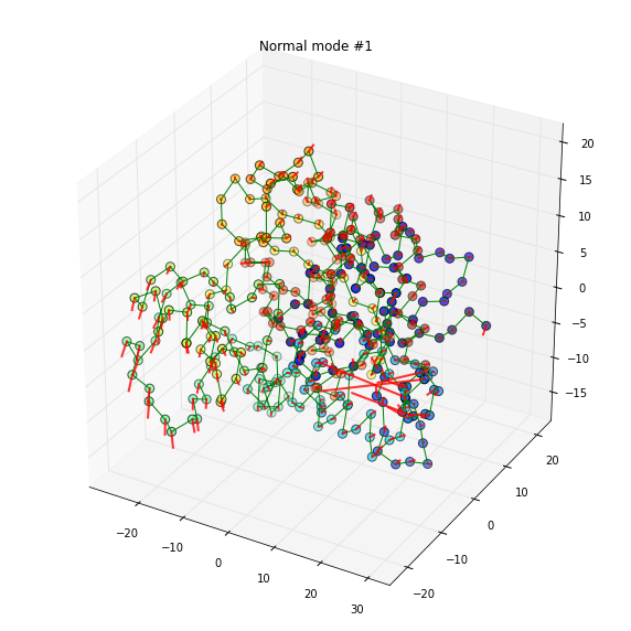

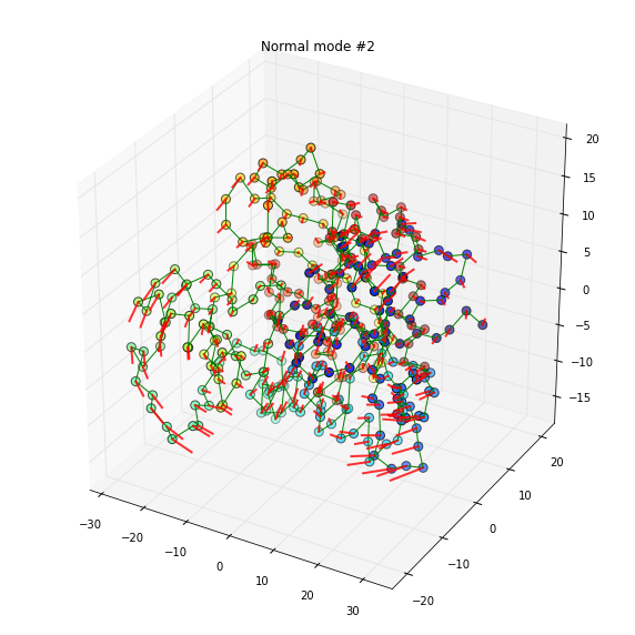
png

The first mode is predominated by the movement of a losely connected loop. The 2nd mode arises a more correlated global motion.

Below an interpolation along the second mode:

png

If you want to ask me a question or leave me a message add @bougui505 in your comment.