Adaptive sampling of a 2D surface potential by Markov Chain Monte Carlo with python
The code below reproduce an example given in the folding@home web site.
%pylab inline
import matplotlib.gridspec as gridspec
import sys
sys.path.append('/Bis/home/bougui/bin/SOM')
import SOMTools
import sklearn.cluster
import scipy.spatial.distance
The sampled potential
First we define a Müller potential as the sampled potential:
def muller_potential(x, y, use_numpy=False):
    """Muller potential
    Parameters
    ----------
    x : {float, np.ndarray, or theano symbolic variable}
    X coordinate. If you supply an array, x and y need to be the same shape,
    and the potential will be calculated at each (x,y pair)
    y : {float, np.ndarray, or theano symbolic variable}
    Y coordinate. If you supply an array, x and y need to be the same shape,
    and the potential will be calculated at each (x,y pair)

    Returns
    -------
    potential : {float, np.ndarray, or theano symbolic variable}
    Potential energy. Will be the same shape as the inputs, x and y.
    Reference
    ---------
    Code adapted from https://cims.nyu.edu/~eve2/ztsMueller.m
    """
    aa = [-1, -1, -6.5, 0.7]
    bb = [0, 0, 11, 0.6]
    cc = [-10, -10, -6.5, 0.7]
    AA = [-200, -100, -170, 15]
    XX = [1, 0, -0.5, -1]
    YY = [0, 0.5, 1.5, 1]
    # use symbolic algebra if you supply symbolic quantities
    exp = np.exp
    value = 0
    for j in range(0, 4):
        if use_numpy:
            value += AA[j] * numpy.exp(aa[j] * (x - XX[j])**2 + bb[j] * (x - XX[j]) * (y - YY[j]) + cc[j] * (y - YY[j])**2)
        else: # use sympy
            value += AA[j] * sympy.exp(aa[j] * (x - XX[j])**2 + bb[j] * (x - XX[j]) * (y - YY[j]) + cc[j] * (y - YY[j])**2)
    return value
The potential is plotted below:
minx=-1.5
maxx=1.2
miny=-0.2
maxy=2
ax=None
grid_width = max(maxx-minx, maxy-miny) / 200.0
xx, yy = np.mgrid[minx : maxx : grid_width, miny : maxy : grid_width]
V = muller_potential(xx, yy, use_numpy=True)
contourf(xx, yy, ma.masked_array(V.clip(max=200), V>inf), 40)
colorbar()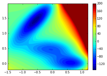
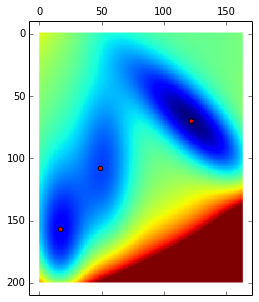
The code below find the 3 local minimum of the potential:
matshow(V.clip(max=200))
lm = asarray(SOMTools.detect_local_minima(V)).T # local minima
scatter(lm[:,1], lm[:,0], c='r')
print lm
[[ 70 122]
[108 49]
[157 17]]
The Monte Carlo sampler
def montecarlo(potential=V, nstep=1000, beta=1, markov=True, start = None):
    p = lambda x: exp(-beta*x)
    nx,ny = potential.shape
    if start == None:
        pos_prev = (np.random.randint(0,nx), np.random.randint(0,ny))
    else:
        pos_prev = start
    traj = []
    for i in range(nstep):
        if markov:
            pos = (pos_prev + asarray([random.choice([-1,0,1]), random.choice([-1,0,1])]))%(nx,ny)
        else:
            pos = (np.random.randint(0,nx), np.random.randint(0,ny))
        pos = tuple(pos)
        pos_prev = tuple(pos_prev)
        delta = potential[pos] - potential[pos_prev]
        if delta > 0:
            #print p(delta)
            if p(delta) < np.random.uniform():
                pos = pos_prev
            else:
                pos_prev = pos
        else:
            pos_prev = pos
        traj.append(pos)
    return asarray(traj)
We define here the number of parallel trajectories to run for the adaptive
sampling (nclone), the number of clusters to define (nstates), the number of
round to perform (nround) and the number of MCMC steps per round (nstep).
nclone = 2
nstates = 3
nround = 10
nstep=50000
The standard trajectory
nstep = nclone*nround*nstep
beta = 0.125
start = lm[-1]
traj_unique = montecarlo(nstep=nstep, beta=beta, start=start)
def get_density(traj):
    density = zeros_like(V)
    for pos in traj:
        pos = tuple(pos)
        density[pos] += 1
    return density
density_unique = get_density(traj_unique)
The obtained distribution looks like:
rcParams['figure.figsize'] = 20,5
contour(V.clip(max=200), 15)
imshow(density_unique / nstep, cmap=cm.coolwarm, norm=matplotlib.colors.LogNorm(), interpolation='nearest')
axis('off')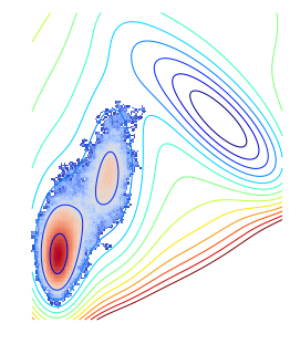
The adaptive sampling
We start from the nclone*nstep first frames of the standard trajectory
trajs = [traj_unique[r*nstep:(r+1)*nstep] for r in range(nclone)]
#print asarray(trajs).shape
all_traj = asarray(trajs).reshape(nclone*nstep,2)
kmeans = sklearn.cluster.KMeans(n_clusters=nstates)
kmeans.fit(all_traj)
starts = asarray([tuple(int_(all_traj[kmeans.labels_==i].mean(axis=0))) for i in unique(kmeans.labels_)])
for r in range(1,nround):
    for i in range(nclone):
        traj = montecarlo(nstep=nstep, beta=beta, start=starts[i])
        trajs.append(traj)
    #print asarray(trajs).shape
    all_traj = asarray(trajs).reshape(nclone*(r+1)*nstep,2)
    kmeans = sklearn.cluster.KMeans(n_clusters=nstates)
    #kmeans.fit(asarray(trajs[::-1][:nclone]).reshape(nclone*nstep,2))
    kmeans.fit(all_traj)
    starts_prev = starts
    starts = asarray([tuple(int_(all_traj[kmeans.labels_==i].mean(axis=0))) for i in unique(kmeans.labels_)])
    #print starts
    starts = starts[scipy.spatial.distance.cdist(starts, starts_prev).min(axis=1).argsort()[::-1]][:nclone]
    print r,starts
1 [[119 46]
[160 16]]
2 [[145 18]
[115 47]]
3 [[ 66 118]
[154 17]]
4 [[112 45]
[ 68 120]]
5 [[154 17]
[110 45]]
6 [[ 68 120]
[111 45]]
7 [[154 17]
[110 45]]
8 [[ 68 120]
[108 46]]
9 [[154 17]
[108 46]]
The obtained distribution with the clustering looks like:
density_all = get_density(all_traj)
max_density = density_all.max()

rcParams['figure.figsize'] = 18,5
nx,ny=V.shape
mgrid = asarray(np.meshgrid(range(nx), range(ny))).T.reshape(nx*ny,2)
contour(V.clip(max=200), 15)
axis('off')
#plot(trajs[i][:,1], trajs[i][:,0])
kmeans = sklearn.cluster.KMeans(n_clusters=3)
kmeans.fit(all_traj)
kmeans_partition = kmeans.predict(mgrid).reshape(nx,ny)
imshow(density_all / max_density, cmap=cm.coolwarm, norm=matplotlib.colors.LogNorm(), interpolation='nearest')
imshow(kmeans_partition, interpolation='none', alpha=0.5)
centers = asarray([tuple(all_traj[kmeans.labels_==i].mean(axis=0)) for i in unique(kmeans.labels_)])
scatter(centers[:,1], centers[:,0], c = range(len(centers)), s=80)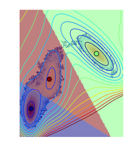
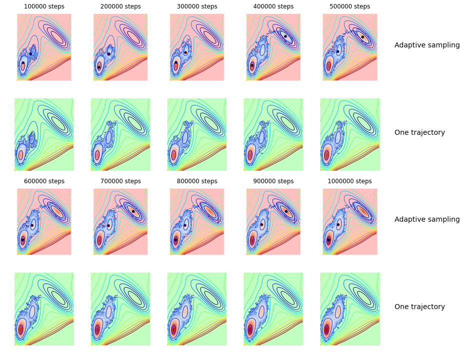
Now we plot the distribution for each round of adaptive sampling and the starting points for the next round. In comparison we plot the evolution of the standard trajectory:
trajs = []

starts = [lm[-1],]*nclone
total_step = nstep*nclone*nround

densities = []
starts_list = []

for r in range(nround):
    trajs.append(all_traj[r*nstep*nclone:(r+1)*nstep*nclone])
    subtraj = asarray(trajs).reshape(nclone*(r+1)*nstep,2)
    kmeans = sklearn.cluster.KMeans(n_clusters=nstates)
    kmeans.fit(subtraj)
    starts_prev = starts
    starts = asarray([tuple(int_(subtraj[kmeans.labels_==i].mean(axis=0))) for i in unique(kmeans.labels_)])
    starts = starts[scipy.spatial.distance.cdist(starts, starts_prev).min(axis=1).argsort()[::-1]][:nclone]
    density = get_density(subtraj)
    densities.append(density)
    starts_list.append(starts)

rcParams['figure.figsize'] = 16,12
gs=gridspec.GridSpec(4,6)
bg1 = zeros((nx,ny,3))
bg1[:,:,0] = 1
bg2 = zeros((nx,ny,3))
bg2[:,:,1] = 1
u=0
v=0
trajs = []
for i, density in enumerate(densities):
    trajs.append(traj_unique[i*nstep*nclone:(i+1)*nstep*nclone])
    #print asarray(trajs).shape
    subtraj = asarray(trajs).reshape(nclone*(i+1)*nstep,2)
    sub_density = get_density(subtraj)
    subplot(gs[u+1,v])
    imshow(bg2, alpha=.25)
    contour(V.clip(max=200), 15)
    imshow(sub_density/max_density, cmap=cm.coolwarm, norm=matplotlib.colors.LogNorm(), interpolation='nearest', vmax=1)
    axis('off')
    starts = starts_list[i]
    subplot(gs[u,v])
    imshow(bg1, alpha=.25)
    contour(V.clip(max=200), 15)
    imshow(density/max_density, cmap=cm.coolwarm, norm=matplotlib.colors.LogNorm(), interpolation='nearest', vmax=1)
    scatter(starts[:,1], starts[:,0], c = range(len(starts)))
    title('%d steps'%((i+1)*nstep*nclone))
    axis('off')
    v+=1
    if v == 5:
        subplot(gs[u,v])
        text(0,0.5,'Adaptive sampling', fontsize=14)
        axis('off')
        subplot(gs[u+1,v])
        text(0,0.5,'One trajectory', fontsize=14)
        axis('off')
        v = 0
        u += 2