New publication: An automatic tool to analyze and cluster macromolecular conformations based on Self-Organizing Maps
Link to the online publication.
Abstract:
Motivation: Sampling the conformational space of biological macromolecules generates large sets of data with considerable complexity. Data-mining techniques, such as clustering, can extract meaningful information. Among them, the Self-Organizing Maps (SOMs) algorithm has shown great promise, in particular since its computation time rises only linearly with the size of the data set. Whereas SOMs are generally used with few neurons, we investigate here their behavior with large numbers of neurons.
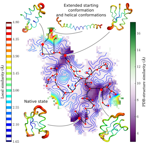
Results: We present here a python library implementing the full SOM analysis workflow. Large SOMs can readily be applied on heavy data sets. Coupled with visualization tools they have very interesting properties. Descriptors for each conformation of a trajectory are calculated and mapped onto a 3D landscape, the U-matrix, reporting the distance between neighboring neurons. To delineate clusters, we developed the flooding algorithm, which hierarchically identifies local basins of the U-matrix from the global minimum to the maximum.
Availability: The python implementation of the SOM library is freely available on github.
Some technical remarks on how the figure has been generated…
Compute the descriptors from the trajectory in dcd format
We start from the DCD trajectory file (traj.dcd) of the folding trajectory of the G protein.
Only the atoms were kept.
This is sufficient for the conformational clustering.
First we create a configuration file (makeVectorsFromdcd_PCA.conf) for the python script applications/makeVectorsFromdcd_PCA.py with the following content:
nframes: the number of framesstructFile: the pdb of your structureprojection: set to TruenProcess: the number of parallel jobs
Below, the makeVectorsFromdcd_PCA.conf file:
[makeVectors]
nframes: 750000
structFile: struct.pdb
trajFile: traj.dcd
projection: True
nProcess: 2
Now, we can run the script:
$ python makeVectorsFromdcd_PCA.py makeVectorsFromdcd_PCA.conf
To generate the conformational descriptors for each frame of the trajectory as described in the publication.
Learn the SOM
Now we can open an interactive python session with ipython or ipython notebook, for example, and import the required python modules.
import numpy
import SOM2
import SOMclust
import SOMTools
from mpl_toolkits.axes_grid1 import make_axes_locatable
from matplotlib import rc
import matplotlib.pyplot as plt
font = {'family' : 'normal', 'size' : 14}
rc('font', **font)
rc('text', usetex=True)
% pylab inline # if you use ipython notebook
Then, we load the input matrix containing the conformational descriptors.
After that we can learn the SOM with som.learn.
inputmatrix = numpy.load('projections.npy')
som = SOM2.SOM(inputmatrix)
som.learn(verbose=True)
smap = som.smap # The SOM map
numpy.save('smap', smap) # We save the SOM map (smap) as a numpy file (npy format)
The U-matrix
Now we can compute the U-matrix corresponding to the map:
nres = smap.shape[-1] / 4 # this line give the number of residue (C alpha)
umat1, umat2, umat3, umat4 = SOMTools.getUmatrix(smap[:,:,:nres]), SOMTools.getUmatrix(smap[:,:,nres:2*nres]), SOMTools.getUmatrix(smap[:,:,2*nres:3*nres]), SOMTools.getUmatrix(smap[:,:,3*nres:4*nres])
umat = (numpy.sqrt(umat1)+numpy.sqrt(umat2)+numpy.sqrt(umat3)+numpy.sqrt(umat4))/nres
We decompose the U-matrix according to the four eigenvectors to compute the U-matrix in Angstrom.
The Best Matching Units (BMUs)
The BMUs give the coordinate of each frame in the SOM map. They allow the projection of data onto the map.
bmus = som.get_allbmus_kdtree()We use the k-d tree algorithm to compute the BMUs to avoid memory errors.
The density
The density gives the number of frame for each unit of the SOM map. It is easily computed from the BMUs:
density = numpy.zeros_like(umat)
for e in bmus:
    density[tuple(e)] += 1
Data projection
In the publication we project the RMSD onto the map. You can compute the RMSD with the program of your choice and then save the data in a text file (one column and one value per line for each frame). This part is very flexible, you can project any property you want.
data = numpy.genfromtxt("data.txt")
projectmap = numpy.zeros_like(umat)
for i, e in enumerate(bmus):
    projectmap[tuple(e)] += data[i]
projectmap /= density
Flooding the map
The SOM map has periodic boundaries. To deal with the periodicity, the flooding algorithm is used. See the publication for more details. Below is the code to flood the map and unwrap it:
clust = SOMclust.clusters(umat, bmus, smap)
clust.getclusters()
Plot the U-matrix and projection with matplotlib
ax = plt.subplot(111)
ax.axis('off')
im1 = ax.contour(numpy.ma.masked_array(clust.umat_cont, clust.mask), 10)
divider = make_axes_locatable(ax)
cax = divider.append_axes("left", size="5%", pad=0.5)
cb1 = plt.colorbar(im1, cax=cax)
cb1.ax.get_children()[4].set_linewidths(18.0) # for the line width in the colorbar of the contour plot
cb1.set_label("Local similarity (\AA)", labelpad=-70)
im2 = ax.imshow(numpy.ma.masked_array(clust.flood(projectmap)[0], clust.mask), interpolation='nearest', cmap=plt.cm.PRGn)
cax = divider.append_axes("right", size="5%", pad=0.1)
cb2 = plt.colorbar(im2, cax=cax)
cb2.set_label("PDB-structre similarity (\AA)")
im3 = ax.scatter(clust.localminima[1], clust.localminima[0], color='r')
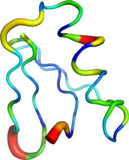
plt.savefig('map.pdf') Sausage representation of an ensemble of structures from rmsf values with pymol
The sausage representations were obtained with pymol.
sausage.py
#!/usr/bin/env python
# -*- coding: UTF8 -*-
"""
author: Guillaume Bouvier
email: guillaume.bouvier@ens-cachan.org
creation date: 2014 07 24
license: GNU GPL
Please feel free to use and modify this, but keep the above information.
Thanks!
"""

import sys
sys.path.append('/c5/shared/pymol/1.7.0.0-python-2.7.5-shared/lib/python2.7/site-packages/')

import __main__
#__main__.pymol_argv = ['pymol','-qc'] # Pymol: quiet and no GUI
import pymol
pymol.finish_launching()

import align_all
import rmsf_states

pdb_file_1 =sys.argv[1]
pdb_name_1 =pdb_file_1.split('.')[0]
pdb_file_2 =sys.argv[2]
pdb_name_2 =pdb_file_2.split('.')[0]

pymol.cmd.load(pdb_file_1, pdb_name_1)
pymol.cmd.disable("all")
pymol.cmd.enable(pdb_name_1)


pymol.cmd.load(pdb_file_2, pdb_name_2)
pymol.cmd.disable("all")
pymol.cmd.enable(pdb_name_2)

print pymol.cmd.get_names()

align_all.align_all(pdb_name_1)

pymol.cmd.hide('all')
pymol.cmd.show('cartoon')

rmsf_states.rmsf_states(pdb_name_2)

pymol.cmd.cartoon('putty')
pymol.cmd.spectrum('b', selection='%s and name CA'%pdb_name_2)

pymol.cmd.orient(pdb_name_2)

pymol.cmd.set('ray_opaque_background', 0)
print "Press enter key to continue or x + enter to terminate"
wait=raw_input()
pymol.cmd.png("%s.png"%(pdb_name_2), width=2400, ray=1)
print 'done'
pymol.cmd.quit()
This script requires these pymol scripts:
align_all.py
#! /usr/bin/env python
# original Written by Jules Jacobsen (jacobsen@ebi.ac.uk). Feel free to do whatever you like with this code.
# extensively modified by Robert L. Campbell (rlc1@queensu.ca)

from pymol import cmd

def align_all(target=None,mobile_selection='name ca',target_selection='name ca',cutoff=2, cycles=5,cgo_object=0):
  """
  Aligns all models in a list to one target

  usage:
    align_all [target][target_selection=name ca][mobile_selection=name ca][cutoff=2][cycles=5][cgo_object=0]
        where target specifies the model id you want to align all others against,
        and target_selection, mobile_selection, cutoff and cycles are options
        passed to the align command.

    By default the selection is all C-alpha atoms and the cutoff is 2 and the
    number of cycles is 5.
    Setting cgo_object to 1, will cause the generation of an alignment object for
    each object.  They will be named like <object>_on_<target>, where <object> and
    <target> will be replaced by the real object and target names.

    Example:
      align_all target=name1, mobile_selection=c. b & n. n+ca+c+o,target_selection=c. a & n. n+ca+c+o

  """
  cutoff = int(cutoff)
  cycles = int(cycles)
  cgo_object = int(cgo_object)

  object_list = cmd.get_names()
  object_list.remove(target)

  rmsd = {}
  rmsd_list = []
  for i in range(len(object_list)):
    if cgo_object:
      objectname = 'align_%s_on_%s' % (object_list[i],target)
      rms = cmd.align('%s & %s'%(object_list[i],mobile_selection),'%s & %s'%(target,target_selection),cutoff=cutoff,cycles=cycles,object=objectname)
    else:
      rms = cmd.align('%s & %s'%(object_list[i],mobile_selection),'%s & %s'%(target,target_selection),cutoff=cutoff,cycles=cycles)

    rmsd[object_list[i]] = (rms[0],rms[1])
    rmsd_list.append((object_list[i],rms[0],rms[1]))

  rmsd_list.sort(lambda x,y:cmp(x[1],y[1]))
# loop over dictionary and print out matrix of final rms values
  print "Aligning against:",target
  for object_name in object_list:
    print "%s: %6.3f using %d atoms" % (object_name,rmsd[object_name][0],rmsd[object_name][1])

  print "\nSorted from best match to worst:"
  for r in rmsd_list:
    print "%s: %6.3f using %d atoms" % r

cmd.extend('align_all',align_all)
rmsf_states.py
#! /usr/bin/python
# Copyright (c) 2009 Robert L. Campbell (rlc1@queensu.ca)
import math,sys
from pymol import cmd
from pymol import stored

def distx2(x1,x2):
  """
  Calculate the square of the distance between two coordinates.
  Returns a float
  """
  distx2 = (x1[0]-x2[0])**2 + (x1[1]-x2[1])**2 + (x1[2]-x2[2])**2
  return distx2


def rmsf_states(selection,byres=0,reference_state=1):
  """
  AUTHOR

    Robert L. Campbell

  USAGE

    rmsf_states selection [,byres=0], [reference_state=1]

    Calculate the RMS fluctuation for each residue in a set of models
    (within a multi-state object).

    If you specify byres=1, then it will only calculate the RMSF for alpha-carbons (i.e.
    it modifies the selection by adding "and name CA"), but will modify the B-factors for
    all atoms in each residue to be the same as the alpha-carbons.

    If you use a selection that only includes only some atoms, only those atoms will have
    their B-factors modified (even with byres=1 specified).

    By default, the RMSF is calculated with respect to the first state, but you can
    change this by specifying setting reference_state to the number of another state.
  """

# setting byres to true only makes sense if the selection is only for the alpha-carbons
  byres = int(byres)
  reference_state = int(reference_state)

# initialize the arrays used
  models = []
  coord_array = []
  chain=[]
  resi=[]
  resn=[]
  name=[]

  num_states = cmd.count_states(selection)

# get models into models array
  for i in range(num_states):
    models.append(cmd.get_model(selection,state=i+1))

# extract coordinates and atom identification information out of the models
# loop over the states
  for i in range(num_states):
    coord_array.append([])
    chain.append([])
    resi.append([])
    resn.append([])
    name.append([])

    if byres:
# loop over the atoms in each state
      for j in range(len(models[0].atom)):
        atom = models[i].atom[j]
        if atom.name == 'CA':
          coord_array[i].append(atom.coord)
          chain[i].append(atom.chain)
          resi[i].append(atom.resi)
          resn[i].append(atom.resn)
          name[i].append(atom.name)
    else:
# loop over the atoms in each state
      for j in range(len(models[0].atom)):
        atom = models[i].atom[j]
        coord_array[i].append(atom.coord)
        chain[i].append(atom.chain)
        resi[i].append(atom.resi)
        resn[i].append(atom.resn)
        name[i].append(atom.name)

# initialize array
  diff2 = []

# calculate the square of the fluctuation
# = the sum of the distance between the atoms in each state from the reference state, squared
  for j in range(len(coord_array[0])):
    diff2.append(0.)
    for i in range(num_states):

# reference_state is 1-based, but coord_array is zero-based, so subtract 1 from
# reference_state to get the correct reference_state
      diff2[j] += distx2(coord_array[i][j],coord_array[reference_state - 1][j])

# divide the fluctuation squared by the number of states and take the square root of that to get the RMSF
    diff2[j] = math.sqrt(diff2[j]/num_states)

# reset all the B-factors to zero
  cmd.alter(selection,"b=0")

  b_dict = {}

  sum_rmsf = 0
# if byres, alter all B-factors in a residue to be the same
  if byres:
    def b_lookup(chain, resi, name):
      if chain in b_dict:
        b = b_dict[chain][resi]
      else:
        b = b_dict[''][resi]
      return b
    stored.b = b_lookup

    for i in range(len(diff2)):
      sum_rmsf += diff2[i]
      b_dict.setdefault(chain[0][i], {})[resi[0][i]] = diff2[i]
    mean_rmsf = sum_rmsf/len(diff2)
    cmd.alter(selection,'%s=stored.b(chain,resi,name)' % ('b'))

# if not byres, alter all B-factors individually according to the RMSF for each atom
  else:
    quiet=0
    def b_lookup(chain, resi, name):
      if chain in b_dict:
        b = b_dict[chain][resi][name]
      else:
        b = b_dict[''][resi][name]
      return b
    stored.b = b_lookup

    for i in range(len(diff2)):
      sum_rmsf += diff2[i]
      try:
        b_dict.setdefault(chain[0][i], {}).setdefault(resi[0][i], {})[name[0][i]] = diff2[i]
      except KeyError:
        print chain[0][i],resi[0][i],name[0][i]
    cmd.alter(selection,'%s=stored.b(chain,resi,name)' % ('b'))
    mean_rmsf = sum_rmsf/len(diff2)

  print "Mean RMSF for selection: %s = %g" % (selection, mean_rmsf)

cmd.extend("rmsf_states",rmsf_states)