WHAM: The Weighted Histogram Analysis Method

First of all, a good introduction to the WHAM method can be found here or here for a local copy.

Sometime, it’s necessary to determine properties from combined simulations under different conditions. The WHAM method allows to unbias the distribution of the combined simulations.

Here, we present the result on a 1D toy model sampled with a Markov Chain Monte Carlo (MCMC)

Here the import in the ipython notebook:

%pylab inline
import matplotlib.gridspec as gridspec
import scipy.optimize as optim

The 1D potential is constructed with a 1D polynomial fit of some points

x = linspace(0,100,7)
y = [5, 1.5, 4, 1, 2, 1.5,5]

plot(x,y,'o')
z = np.polyfit(x, y, 6)
E = np.poly1d(z)

x_lin = linspace(0, 100, 100)
plot(x_lin,E(x_lin), linewidth=2)
ylabel('Potential', fontsize=18)
xlabel('discrete coordinates', fontsize=18)
grid()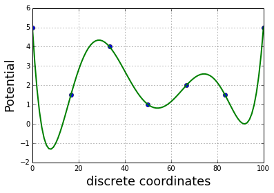

png

This potential is then sampled using a MCMC

def montecarlo(potential=E, nstep=1000, beta=1):
    p = lambda x: exp(-beta*x)
    pos_prev = random.randint(0,100)
    traj = []
    for i in range(nstep):
        pos = pos_prev + randint(0, 2)*2 -1
        while not (0 <= pos < 100):
            pos = pos_prev + randint(0, 2)*2 -1
        delta = potential(pos) - potential(pos_prev)
        if delta > 0:
            #print p(delta)
            if p(delta) < random.uniform():
                pos = pos_prev
            else:
                pos_prev = pos
        else:
            pos_prev = pos
        #print pos, pos_prev, delta, potential(pos), potential(pos_prev)
        traj.append(pos)
    return asarray(traj)

We used six different temperature ($T=\beta^{-1}$):

$\beta=1.00$
$\beta=0.85$
$\beta=0.70$
$\beta=0.55$
$\beta=0.40$
$\beta=0.25$

beta_list = linspace(1,0.25,6)
traj_list = []
for beta in beta_list:
    traj_list.append(montecarlo(nstep=100000, beta=beta))

And then we plot the distributions obtained from the 6 MCMC:

rcParams['figure.figsize'] = 16,8
gs = gridspec.GridSpec(2,3)
i,j = 0,0
for c,traj in enumerate(traj_list):
    subplot(gs[i,j])
    title(r'$\beta$ = %.2f'%beta_list[c], fontsize=18)
    if j == 0:
        ylabel('$\pi$', fontsize=18)
    if i == 1:
        xlabel('discrete coordinates', fontsize=18)
    grid()
    tmp = hist(traj, 100, normed=True)

    twinx()
    plot(x_lin,E(x_lin), linewidth=2, color='r')
    if j == 2:
        ylabel('Potential', fontsize=18)
    j += 1
    if j == 3:
        j = 0
        i += 1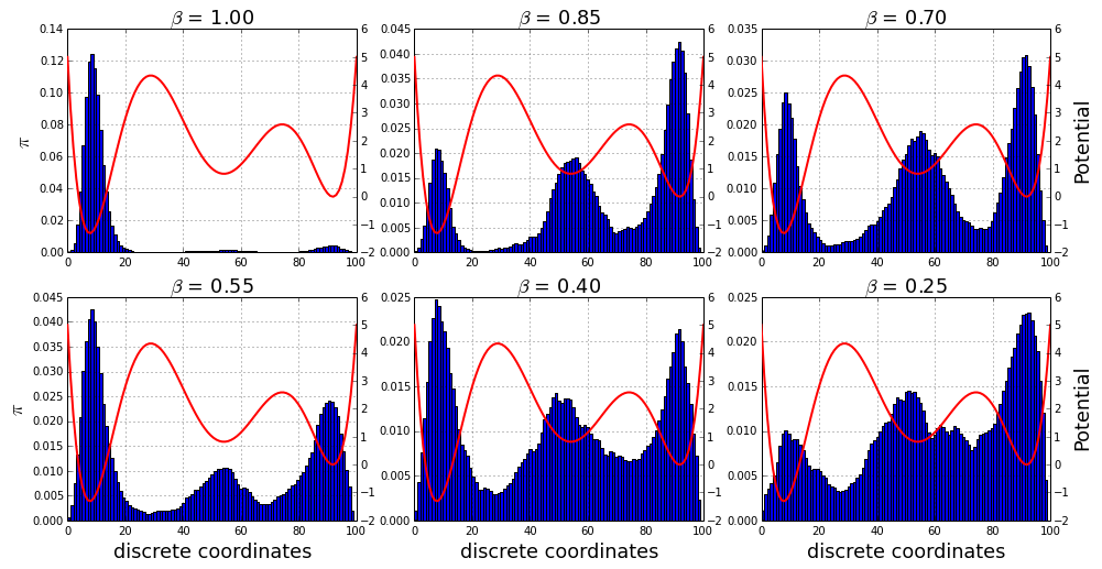

png

We can look at the distribution of the six MCMC simulations merged together:

rcParams['figure.figsize'] = 16/3,8/2
traj_combined = asarray(traj_list).flatten()
tmp = hist(traj_combined, 100, normed=True)
xlabel('discrete coordinates', fontsize=18)
ylabel('$\pi$', fontsize=18)
twinx()
plot(x_lin,E(x_lin), linewidth=2, color='r')
ylabel('Potential', fontsize=18)
tmp = title('Combined trajectory', fontsize=18)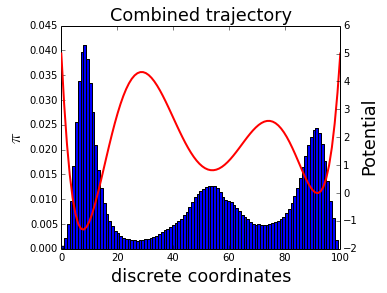

png

This distribution is biased as we run the MCMC at 6 different temperatures. The aim of WHAM is to unbias the distribution. We assume that $p_{ij}$ , the biased probability of bin j in the i-th simulation, is related to $p_{j}$ , the unbiased probability of bin j via:

$p_{ij} = f_{i}c_{ij}p_{j}^{o}$

where $c_{ij}$ is the biasing factor and $f_{i}$ is a normalizing constant chosen such that $\sum_{j}p_{ij}=1$ :

$f_{i} = \frac{1}{\sum_{j}c_{ij}p_{j}^{o}}$

For the temperature biasing:

$c_{ij} = \exp{(-(\beta_{i}-\beta_{0})E_{j})}$

We assume that we want to compute the potential of mean force (PMF) at $\beta=1$.

We can compute $c_{ij}$:

n_sim = len(beta_list) # number of simulations
n_bin = len(x_lin) # number of bins
c = zeros((n_sim, n_bin))
beta0 = 1 # the beta of the unbias distribution we want to compute
for i,beta in enumerate(beta_list):
    for j,e in enumerate(E(x_lin)):
        c[i,j] = exp(-(beta-beta0)*e)

Just for fun, the visualisation of c:

rcParams['figure.figsize'] = 16,5
imshow(c,cmap=cm.coolwarm, norm=matplotlib.colors.LogNorm())
tmp = colorbar()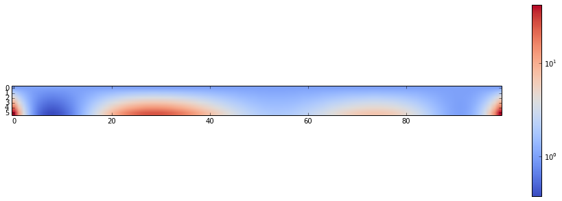

png

An optimal estimate of $p_{j}^{o}$ is given by:

$p_{j}^{o} = \frac{\sum_{i=1}^{S}n_{ij}}{\sum_{i=1}^{S}N_{i}f_{i}c_{ij}}$

with $n_{ij}$ the number of bin count for simulation i and bin j and $N_{i}$ the total number of sample generated by the i-th simulation.

and, as said before:

$f_{i} = \frac{1}{\sum_{j=1}^{M}c_{ij}p_{j}^{o}}$

S is the total number of simulations (here $S=6$) and M is the total number of bins (here $M=100$).

We can easily compute $n_{ij}\;\forall\;(i,j)$

n = zeros((n_sim, n_bin))
for i,traj in enumerate(traj_list):
    n[i] = histogram(traj, bins=100)[0]

A representation of n:

matshow(n, cmap=cm.coolwarm, norm=matplotlib.colors.LogNorm())
tmp = colorbar()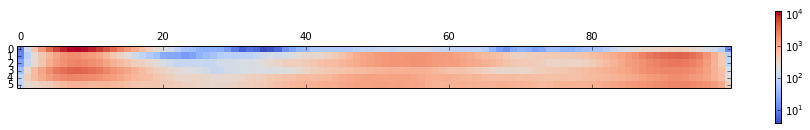

png

Now we use fsolve to solve the WHAM equations described below:

p0_guess = ones(n_bin, float)
f_guess = ones(n_sim, float)
N = asarray([traj.shape[0] for traj in traj_list])
def residual(P):
    p0,f = P[:n_bin],P[n_bin:]
    #print p0.shape, f.shape
    res1 = p0 - n.sum(axis=0)/(N*f*c.T).T.sum(axis=0)
    res2 = f - 1/((c*p0).sum(axis=1))
    return concatenate((res1, res2))
#residual(concatenate((p0_guess,f_guess)))
P = optim.fsolve(residual, concatenate((p0_guess, f_guess)))
#print P.x
p0,f = P[:n_bin],P[n_bin:]

And here the result; the unbias distribution for $\beta=1$

plot(p0)
xlabel('discrete coordinates', fontsize=18)
tmp = ylabel('$\pi$', fontsize=18)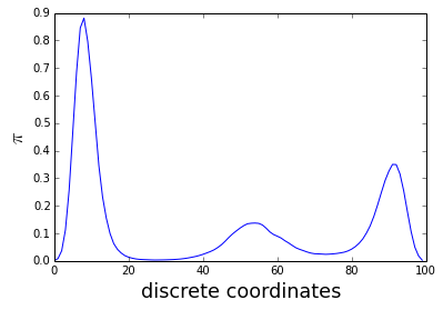

png

We can then derived the free energy profile (F) or Potential of Mean force (PMF):

$F = F_{0} - \frac{1}{\beta}\ln(p^o)$

and compare to the initial one, used in the toy model:

plot(-log(p0), linewidth=2, label='PMF')
plot(x_lin,E(x_lin), linewidth=2, label='Original potential')
ylabel('Potential', fontsize=18)
xlabel('discrete coordinates', fontsize=18)
grid()
tmp = legend()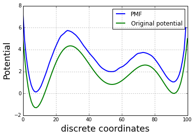

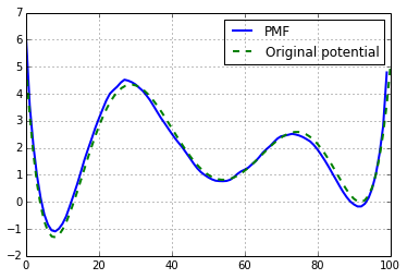
png

If we normalized with the $F_{0}$ factor we obtain:

F0 = (log(p0) + E(x_lin)).mean()
plot(F0-log(p0), linewidth=2, label='PMF')
plot(x_lin,E(x_lin), '--', linewidth=2, label='Original potential')
grid()
tmp = legend()

png

If you want to ask me a question or leave me a message add @bougui505 in your comment.